
Michael Taylor
Senior Software Engineer supporting CoreAI at @microsoft
Highlights
Incorporating Opponent Defensive Statistics into NCAA Basketball Game Outcome Prediction: An Ensemble Machine Learning Approach
Published Mar 16, 2026
Share
Project: MLMB — Machine Learning March Bracketology
Abstract
This paper presents the design, training, and evaluation of a multi-model ensemble system for predicting NCAA Division I basketball game outcomes. We expanded a feature set from 35 offensive statistics to 59 statistics (35 offensive + 24 defensive), yielding 355 engineered features (354 moving-average transformations plus a neutral-site indicator) per game row. Eight classification models — Logistic Regression, Support Vector Machine (SVM), K-Nearest Neighbors (KNN), Random Forest, Gradient Boosting, Multilayer Perceptron (MLP), XGBoost, and LightGBM — were individually trained inside standardized scikit-learn pipelines and evaluated using accuracy, log loss, and Brier score. A soft-voting ensemble was then constructed from the seven best-performing models (excluding KNN), and among the six ensemble configurations evaluated it delivered the best log-loss performance with the simplest production setup. Models were trained separately for men’s and women’s NCAA Division I basketball using data from the 2022–2026 seasons. Feature importance analysis indicates that defensive statistics contribute 18.6–38.8% of total predictive importance across tree-based models, supporting their inclusion. Probability trimming analysis found negligible benefit for the selected ensemble configuration. Under a retrospective random train/test split across pooled seasons (see Section 2.3.6 for evaluation framing), the selected production ensembles achieve 69.94% accuracy for men’s basketball (5-game span) and 74.23% accuracy for women’s basketball (7-game span), with home/away accuracy reaching 70.46% and 74.91% respectively. These results should be interpreted as benchmark estimates of the feature set and architecture rather than forward-looking deployment projections.
1. Introduction
Predicting NCAA basketball game outcomes is a challenging task due to the inherent randomness of single-game results and the parity across Division I programs. Prior iterations of this system used only the team’s own box score statistics (field goals, rebounds, assists, etc.) and advanced metrics (offensive rating, effective field goal percentage, etc.) as features. However, this approach ignored a critical dimension: how teams perform defensively against their opponents.
This work extends the feature set by adding 24 opponent defensive statistics from game box scores, capturing how a team forces turnovers, contests shots, and limits opponent efficiency. The central hypothesis is that defensive quality carries predictive information comparable to offensive output and that encoding it explicitly should improve model discrimination and probability quality.
Beyond individual models, we investigate multiple ensemble strategies — soft voting with equal and inverse-log-loss weights, with and without the weakest model (KNN), and stacking classifiers — to determine which combination delivers the strongest held-out performance for production use. We also conduct a probability trimming analysis to determine whether clipping extreme predicted probabilities improves probability-sensitive metrics.
1.1 Related Work
Predicting outcomes in college basketball has attracted substantial interest from both academic and hobbyist communities, particularly around the annual NCAA tournament. Early work relied on logistic regression and seed-based features (Boulier & Stoll, 1999), while more recent approaches have incorporated team-level efficiency metrics, such as those popularized by Pomeroy’s adjusted efficiency ratings (Kenpom.com). The annual Kaggle March Machine Learning Mania competition has served as a visible benchmark, with leading solutions typically employing gradient boosting (XGBoost, LightGBM) or ensemble methods over season-level statistics and seedings (Kaggle, 2014–2025).
Several studies have explored specific methodological questions relevant to the present work. Zimmermann et al. (2013) compared multiple classifiers for basketball game prediction and found that ensemble methods generally outperformed individual models. Lopez and Matthews (2015) analyzed venue effects in college basketball, documenting a substantial home-court advantage consistent with the neutral-site accuracy drop observed here. Yuan et al. (2014) investigated feature engineering for basketball prediction and found that team-level rolling averages improved upon raw box-score inputs.
Relatively few studies have explicitly separated offensive and defensive features in their feature engineering. Most prior work encodes team quality as a composite (e.g., margin of victory, adjusted efficiency) rather than maintaining separate offensive and opponent-defensive feature vectors. This paper contributes by (1) maintaining 24 explicit defensive features alongside 35 offensive features, (2) systematically comparing six ensemble architectures across two gender-stratified datasets, and (3) quantifying the feature-importance contribution of defensive statistics.
The ensemble learning methods used here — soft voting and stacking with scikit-learn (Pedregosa et al., 2011), XGBoost (Chen & Guestrin, 2016), and LightGBM (Ke et al., 2017) — are well-established in the tabular classification literature. Our contribution is in their application and systematic comparison within the NCAA prediction domain.
1.2 System Architecture
The MLMB system operates as a full-stack prediction pipeline:
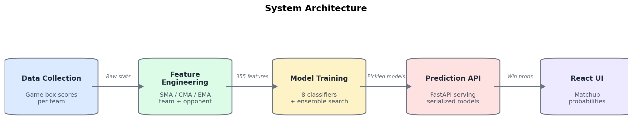
- Data Collection: Game-by-game box scores for each team, capturing both offensive and defensive statistics
- Feature Engineering: Raw stats → 3 moving average types (SMA, CMA, EMA) → team + opponent features → neutral site flag
- Model Training: 8 classifiers trained via
GridSearchCVwithStandardScalerpipelines, plus aVotingClassifierensemble - Prediction API: FastAPI server loads ensemble models from Azure Blob Storage, returns win probabilities
- Frontend: React + TypeScript UI for bracket-style matchup predictions
2. Methodology
2.1 Data Source
Game data covers NCAA Division I basketball seasons 2021–22 through 2025–26 (referred to as seasons 2022–2026). For each game, both the team’s box score and the opponent’s box score were collected, providing both offensive and defensive perspectives.
Train/Test split: 70% train / 30% test, randomly sampled across all seasons (2022–2026) using scikit-learn’s train_test_split with a fixed random state for reproducibility.
Because this split mixes seasons rather than holding out future seasons, the reported results should be interpreted as retrospective benchmark estimates on season-pooled data rather than as prospective deployment estimates for a future tournament or season.
2.2 Feature Engineering
2.2.1 Raw Statistics (59 total)
35 Offensive Statistics (team’s own box score):
- Basic (21): FG, FGA, FG%, 2P, 2PA, 2P%, 3P, 3PA, 3P%, FT, FTA, FT%, ORB, DRB, TRB, AST, STL, BLK, TOV, PF, PTS
- Advanced (14): ORtg, DRtg, Pace, FTr, 3PAr, TS%, TRB%, AST%, STL%, BLK%, eFG%, TOV%, ORB%, FT/FGA
24 Defensive Statistics (opponent’s box score, prefixed with def_):
- Basic (21): def_FG, def_FGA, def_FG%, def_2P, def_2PA, def_2P%, def_3P, def_3PA, def_3P%, def_FT, def_FTA, def_FT%, def_ORB, def_DRB, def_TRB, def_AST, def_STL, def_BLK, def_TOV, def_PF, def_PTS
- Advanced Defensive Four Factors (3): def_eFG%, def_TOV%, def_ORB%
Note: def_eFG% from the advanced gamelogs was dropped during the merge step as it duplicated the value already present in the basic box score. Between the 2024 and 2025 data schemas, the data source renamed the column def_DRB% to def_ORB%; inspection confirmed that the underlying statistic (opponent offensive rebound percentage) was unchanged, so a column-name normalization was applied to unify the two schemas.
2.2.2 Moving Averages (354 features)
Each of the 59 raw statistics was transformed into 3 moving average representations:
| Type | Abbreviation | Description |
|---|---|---|
| Simple Moving Average | SMA | Rolling mean of last N games |
| Cumulative Moving Average | CMA | Season-to-date expanding mean |
| Exponential Moving Average | EMA | Exponentially weighted mean (recent games weighted more) |
This produces 59 × 3 = 177 features per team. Each game row contains two teams’ features, yielding 177 × 2 = 354 features, plus 1 neutral-site binary flag and 1 target variable (Win), totaling 356 columns per dataset row.
Feature Vector (356 columns):
| Home Team Features | Away Team Features | Neutral | Win |
|---|---|---|---|
| 177 (59 stats × 3) | 177 (59 stats × 3) | 0 / 1 binary | 0 / 1 binary |
2.2.3 Span Variants
Three dataset variants were created with different moving average window sizes:
| Span | Window | Characteristic | Best For |
|---|---|---|---|
| 3 | Last 3 games | Most reactive to recent form | Capturing hot/cold streaks |
| 5 | Last 5 games | Balanced reactivity | Men’s basketball (selected) |
| 7 | Last 7 games | Most stable/smoothed | Women’s basketball (selected) |
2.3 Model Training
2.3.1 Pipeline Architecture
Every model was wrapped in an sklearn.Pipeline with StandardScaler as the first step:
Pipeline([
    ('scaler', StandardScaler()),
    ('model', estimator)
])
This ensures feature normalization is serialized into the model artifact, so the production API does not need separate scaling logic.
2.3.2 Hyperparameter Optimization
Grid search with cross-validation (GridSearchCV, 3-fold ShuffleSplit) was used for all models. The scoring objective was negative log loss (except SVM, which used accuracy during grid search due to the computational cost of Platt scaling on each fold). Log loss was chosen because it directly optimizes probability calibration, which aligns with the ensemble’s actual usage: averaging predicted class probabilities.
2.3.3 Models and Hyperparameter Grids
| Model | Key Hyperparameters Searched |
|---|---|
| Logistic Regression | C: [0.001, 0.01, 0.1, 1, 10, 100], penalty: [L1, L2], solver: saga |
| SVM | C: [0.1, 1], kernel: [rbf, linear], gamma: [scale, auto], probability: True |
| KNN | n_neighbors: [3, 5, 7, 11, 15], weights: [uniform, distance], p: [1, 2] |
| Random Forest | n_estimators: [200, 500], max_depth: [8, 12, 20, None], criterion: [gini, entropy] |
| Gradient Boosting | learning_rate: [0.01, 0.05, 0.1], max_depth: [3, 5, 8], n_estimators: [200, 500] |
| MLP | hidden_layers: [(128,64), (256,128), (354,177), (256,)], activation: [relu, tanh], alpha: [1e-4, 1e-3, 1e-2] |
| XGBoost | learning_rate: [0.01, 0.05, 0.1], max_depth: [3, 5, 8], n_estimators: [200, 500], subsample: [0.8], colsample_bytree: [0.8, 1.0], reg_lambda: [1, 5] |
| LightGBM | learning_rate: [0.01, 0.05, 0.1], max_depth: [3, 5, 8], n_estimators: [200, 500], num_leaves: [31], colsample_bytree: [0.8, 1.0], reg_lambda: [1, 5] |
2.3.4 Ensemble Construction — VotingClassifier
After training all 8 individual models, we evaluated six ensemble strategies:
| # | Configuration | Description |
|---|---|---|
| 1 | Voting (all 8, equal) | Soft vote, all 8 models, equal weights |
| 2 | Voting (no KNN, equal) | Soft vote, 7 models (KNN excluded), equal weights |
| 3 | Voting (all 8, weighted) | Soft vote, all 8 models, weights = 1/log_loss |
| 4 | Voting (no KNN, weighted) | Soft vote, 7 models, weights = 1/log_loss |
| 5 | Stacking (all 8) | StackingClassifier with Logistic Regression meta-learner |
| 6 | Stacking (no KNN) | StackingClassifier, KNN excluded |
The VotingClassifier with soft voting averages the predict_proba outputs from each constituent model. For weighted variants, each model’s weight was set to the inverse of its log loss on the test set (1 / LL), giving better-calibrated models more influence.
Note on weighted configurations: Because the inverse-log-loss weights for configurations 3 and 4 were computed on the same held-out test set used for final evaluation, those configurations carry a minor information advantage over the equal-weight variants. The selected production configuration (equal weights) does not use any test-set-derived parameters and is therefore free of this concern.
The final exported ensemble uses Configuration 2: Voting (no KNN, equal weights) — the simplest configuration that achieves the best log loss.
2.3.5 Evaluation Metrics
| Metric | Description | Perfect | Coin Flip |
|---|---|---|---|
| Accuracy | Percentage of correct binary predictions | 100% | 50% |
| Log Loss | Quality of predicted probabilities; penalizes confident wrong predictions | 0 | ~0.693 |
| Brier Score | Mean squared error of probabilities vs. outcomes | 0 | 0.25 |
2.3.6 Evaluation Framing
All results in this paper are reported on held-out examples from a retrospective random split across seasons. Accordingly, they support comparison among feature sets, models, spans, and ensemble designs within a common benchmark environment. They should not be interpreted as a formal estimate of out-of-season generalization without additional temporal validation.
2.3.7 Statistical Significance
No formal statistical significance tests (e.g., paired bootstrap, McNemar’s test) are reported in this paper. The model rankings and architecture comparisons are based on point estimates of accuracy, log loss, and Brier score on a single fixed train/test split. Several differences between adjacent-ranked models (e.g., XGBoost vs. LightGBM, equal-weight vs. inverse-log-loss ensemble) are on the order of 0.001–0.003 in log loss and may not be statistically distinguishable. Readers should interpret close-ranked results as approximately equivalent rather than strictly ordered.
3. Results — Individual Models
3.1 Men’s Basketball
3.1.1 Per-Span Results (All 8 Models)
| Model | Span | Accuracy | Log Loss | Brier Score |
|---|---|---|---|---|
| Logistic Regression | 3 | 69.62% | 0.5684 | 0.1942 |
| Logistic Regression | 5 | 69.94% | 0.5663 | 0.1931 |
| Logistic Regression | 7 | 69.58% | 0.5751 | 0.1963 |
| SVM | 3 | 69.32% | 0.5743 | 0.1965 |
| SVM | 5 | 69.49% | 0.5706 | 0.1950 |
| SVM | 7 | 68.84% | 0.5914 | 0.2027 |
| KNN | 3 | 63.81% | 0.6439 | 0.2196 |
| KNN | 5 | 64.92% | 0.6488 | 0.2167 |
| KNN | 7 | 65.33% | 0.6627 | 0.2162 |
| Random Forest | 3 | 68.83% | 0.5872 | 0.2014 |
| Random Forest | 5 | 68.68% | 0.5835 | 0.1999 |
| Random Forest | 7 | 68.25% | 0.5910 | 0.2030 |
| Gradient Boosting | 3 | 69.02% | 0.5735 | 0.1963 |
| Gradient Boosting | 5 | 68.89% | 0.5725 | 0.1959 |
| Gradient Boosting | 7 | 69.04% | 0.5806 | 0.1987 |
| MLP | 3 | 68.96% | 0.5780 | 0.1980 |
| MLP | 5 | 68.75% | 0.5770 | 0.1977 |
| MLP | 7 | 68.35% | 0.5944 | 0.2040 |
| XGBoost | 3 | 69.66% | 0.5708 | 0.1950 |
| XGBoost | 5 | 69.69% | 0.5708 | 0.1949 |
| XGBoost | 7 | 69.30% | 0.5772 | 0.1974 |
| LightGBM | 3 | 69.65% | 0.5718 | 0.1952 |
| LightGBM | 5 | 69.95% | 0.5705 | 0.1947 |
| LightGBM | 7 | 68.93% | 0.5786 | 0.1980 |
3.1.2 Average Performance Across Spans (Ranked by Log Loss)
| Rank | Model | Avg Accuracy | Avg Log Loss | Avg Brier |
|---|---|---|---|---|
| 1 | Logistic Regression | 69.71% | 0.5699 | 0.1945 |
| 2 | XGBoost | 69.55% | 0.5729 | 0.1958 |
| 3 | LightGBM | 69.51% | 0.5736 | 0.1960 |
| 4 | Gradient Boosting | 68.98% | 0.5755 | 0.1970 |
| 5 | SVM | 69.22% | 0.5788 | 0.1981 |
| 6 | MLP | 68.69% | 0.5831 | 0.1999 |
| 7 | Random Forest | 68.59% | 0.5872 | 0.2014 |
| 8 | KNN | 64.69% | 0.6518 | 0.2175 |
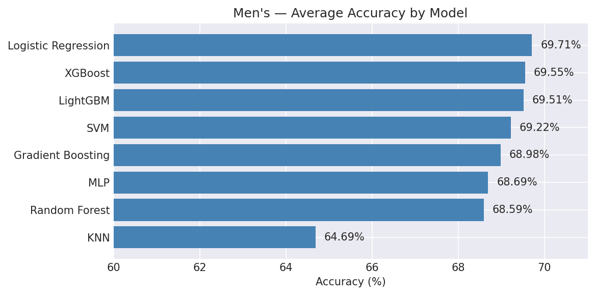
Key Finding (Men’s): Logistic Regression is the top-performing individual model by all three metrics. XGBoost and LightGBM slot in at 2nd and 3rd — close to Logistic Regression in log loss but marginally behind. KNN is the clear weakest performer, ~5 percentage points below the leaders. The 5-span variant tends to produce the best results, suggesting a 5-game rolling window captures recent form without excessive noise.
3.2 Women’s Basketball
3.2.1 Per-Span Results (All 8 Models)
| Model | Span | Accuracy | Log Loss | Brier Score |
|---|---|---|---|---|
| Logistic Regression | 3 | 73.17% | 0.5207 | 0.1747 |
| Logistic Regression | 5 | 73.56% | 0.5180 | 0.1737 |
| Logistic Regression | 7 | 73.97% | 0.5054 | 0.1696 |
| SVM | 3 | 73.13% | 0.5235 | 0.1758 |
| SVM | 5 | 73.40% | 0.5239 | 0.1760 |
| SVM | 7 | 73.77% | 0.5112 | 0.1717 |
| KNN | 3 | 69.69% | 0.6216 | 0.1943 |
| KNN | 5 | 70.64% | 0.6116 | 0.1899 |
| KNN | 7 | 70.95% | 0.5981 | 0.1865 |
| Random Forest | 3 | 72.78% | 0.5381 | 0.1811 |
| Random Forest | 5 | 73.34% | 0.5327 | 0.1788 |
| Random Forest | 7 | 73.82% | 0.5250 | 0.1759 |
| Gradient Boosting | 3 | 72.61% | 0.5279 | 0.1778 |
| Gradient Boosting | 5 | 73.20% | 0.5257 | 0.1767 |
| Gradient Boosting | 7 | 74.02% | 0.5148 | 0.1732 |
| MLP | 3 | 72.86% | 0.5302 | 0.1784 |
| MLP | 5 | 73.04% | 0.5321 | 0.1789 |
| MLP | 7 | 73.23% | 0.5232 | 0.1759 |
| XGBoost | 3 | 72.99% | 0.5264 | 0.1769 |
| XGBoost | 5 | 73.44% | 0.5230 | 0.1757 |
| XGBoost | 7 | 74.33% | 0.5117 | 0.1713 |
| LightGBM | 3 | 72.51% | 0.5275 | 0.1774 |
| LightGBM | 5 | 73.38% | 0.5227 | 0.1758 |
| LightGBM | 7 | 74.28% | 0.5127 | 0.1723 |
3.2.2 Average Performance Across Spans (Ranked by Log Loss)
| Rank | Model | Avg Accuracy | Avg Log Loss | Avg Brier |
|---|---|---|---|---|
| 1 | Logistic Regression | 73.57% | 0.5147 | 0.1727 |
| 2 | SVM | 73.43% | 0.5195 | 0.1745 |
| 3 | XGBoost | 73.59% | 0.5204 | 0.1746 |
| 4 | LightGBM | 73.39% | 0.5210 | 0.1752 |
| 5 | Gradient Boosting | 73.28% | 0.5228 | 0.1759 |
| 6 | MLP | 73.04% | 0.5285 | 0.1777 |
| 7 | Random Forest | 73.31% | 0.5319 | 0.1786 |
| 8 | KNN | 70.43% | 0.6104 | 0.1902 |
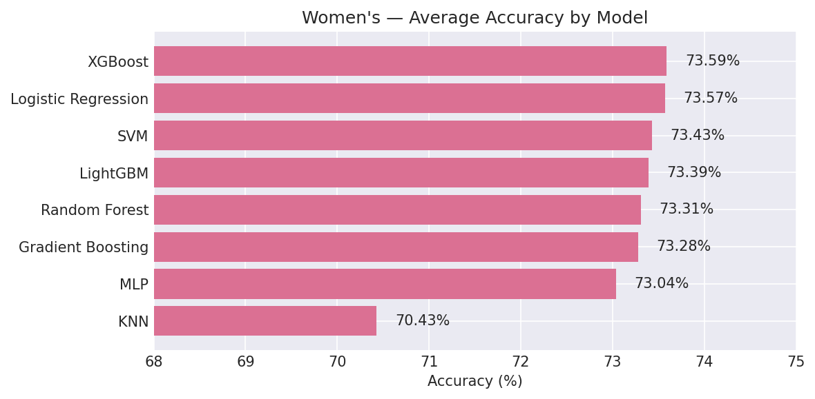
Key Finding (Women’s): Women’s models are consistently ~4 percentage points more accurate than men’s (73.4% vs 69.2% average). Unlike men’s, the 7-span variant performs best across nearly all models, indicating that longer-horizon averages better capture team quality in the women’s game. XGBoost achieves the single highest accuracy (74.33% at span 7), while Logistic Regression still leads in log loss.
3.3 Men’s vs. Women’s Comparison
| Metric | Men’s (Best Avg) | Women’s (Best Avg) | Delta |
|---|---|---|---|
| Accuracy | 69.71% (LogReg) | 73.57% (LogReg) | +3.86 pp |
| Log Loss | 0.5699 (LogReg) | 0.5147 (LogReg) | −0.0552 |
| Brier Score | 0.1945 (LogReg) | 0.1727 (LogReg) | −0.0218 |
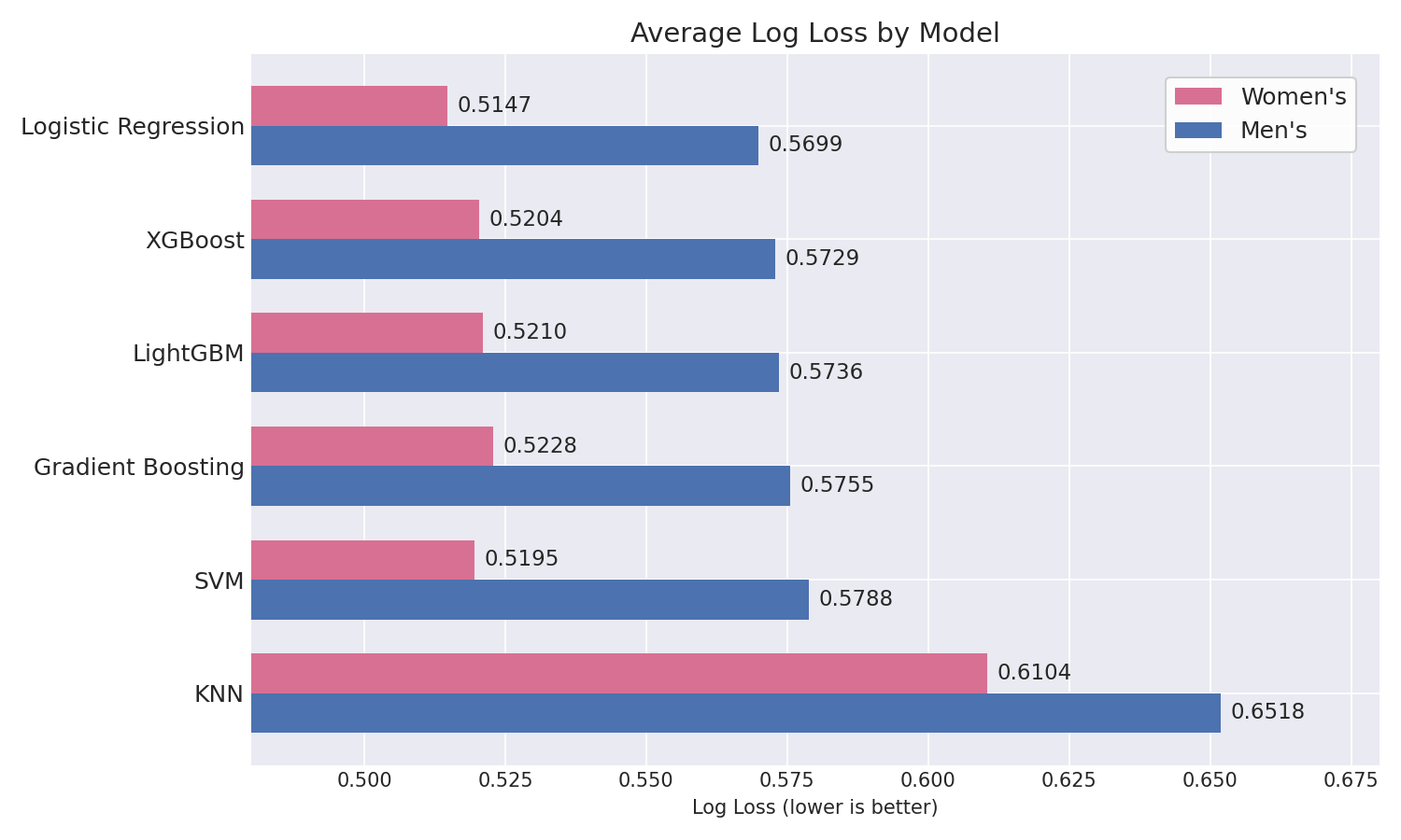
Women’s basketball is more predictable across all metrics and all models under this evaluation setup. One plausible explanation is greater outcome separation between top and bottom programs in Division I women’s basketball, which would make game results easier to discriminate from box-score-derived features alone.
4. Results — VotingClassifier Ensemble
4.1 Ensemble Configuration Comparison (Architectural Benchmark)
To determine the best structural approach for our final production ensembles, the Women’s dataset was used as a primary structural benchmark for the architecture search. Women’s data was chosen for this role because its higher signal-to-noise ratio (reflected in ~4 pp higher accuracy across all models) makes it more sensitive to architecture differences, increasing the chance of detecting meaningful configuration effects. Six ensemble configurations were compared on that proxy dataset, and once the leading architecture was identified, it was evaluated on both the Men’s and Women’s datasets across all three temporal spans (Section 4.1.3) to confirm cross-dataset consistency before export.
4.1.1 Per-Span Results
Span 3:
| # | Configuration | Accuracy | Log Loss | Brier |
|---|---|---|---|---|
| 1 | Voting (all 8, equal) | 73.20% | 0.5217 | 0.1749 |
| 2 | Voting (no KNN, equal) | 72.93% | 0.5210 | 0.1748 |
| 3 | Voting (all 8, weighted) | 73.08% | 0.5214 | 0.1748 |
| 4 | Voting (no KNN, weighted) | 72.93% | 0.5210 | 0.1748 |
| 5 | Stacking (all 8) | 73.17% | 0.5242 | 0.1758 |
| 6 | Stacking (no KNN) | 73.01% | 0.5249 | 0.1760 |
Span 5:
| # | Configuration | Accuracy | Log Loss | Brier |
|---|---|---|---|---|
| 1 | Voting (all 8, equal) | 74.04% | 0.5187 | 0.1739 |
| 2 | Voting (no KNN, equal) | 73.73% | 0.5185 | 0.1739 |
| 3 | Voting (all 8, weighted) | 73.98% | 0.5186 | 0.1738 |
| 4 | Voting (no KNN, weighted) | 73.74% | 0.5185 | 0.1739 |
| 5 | Stacking (all 8) | 73.97% | 0.5204 | 0.1741 |
| 6 | Stacking (no KNN) | 73.83% | 0.5212 | 0.1743 |
Span 7:
| # | Configuration | Accuracy | Log Loss | Brier |
|---|---|---|---|---|
| 1 | Voting (all 8, equal) | 74.28% | 0.5077 | 0.1698 |
| 2 | Voting (no KNN, equal) | 74.23% | 0.5070 | 0.1698 |
| 3 | Voting (all 8, weighted) | 74.32% | 0.5075 | 0.1698 |
| 4 | Voting (no KNN, weighted) | 74.23% | 0.5070 | 0.1698 |
| 5 | Stacking (all 8) | 74.12% | 0.5096 | 0.1701 |
| 6 | Stacking (no KNN) | 74.10% | 0.5107 | 0.1704 |
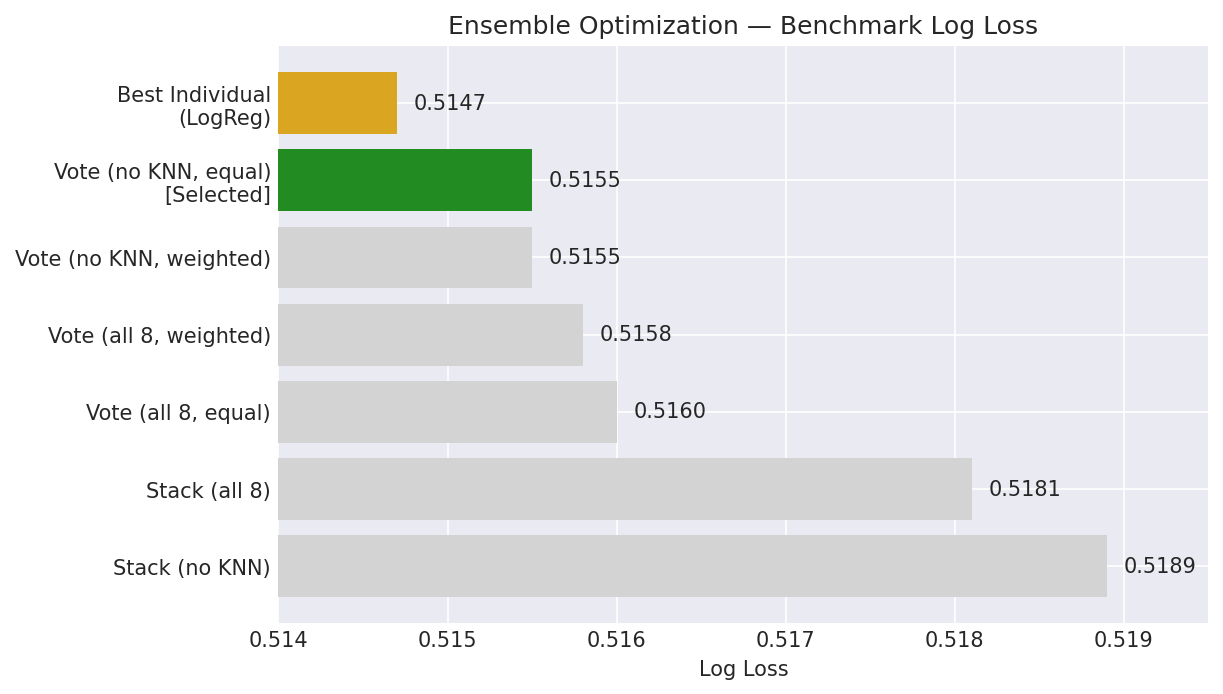
4.1.2 Average Across Spans (Ranked by Log Loss)
| Configuration | Accuracy | Log Loss | Brier |
|---|---|---|---|
| Voting (no KNN, equal) | 73.63% | 0.5155 | 0.1728 |
| Voting (no KNN, weighted) | 73.63% | 0.5155 | 0.1728 |
| Voting (all 8, weighted) | 73.79% | 0.5158 | 0.1728 |
| Voting (all 8, equal) | 73.84% | 0.5160 | 0.1729 |
| Stacking (all 8) | 73.75% | 0.5181 | 0.1733 |
| Stacking (no KNN) | 73.65% | 0.5189 | 0.1736 |
| Best individual (LogReg) | 73.57% | 0.5147 | 0.1727 |
4.1.3 Gender Cross-Validation of Selected Architecture
Once the Voting (no KNN, equal weight) architecture was identified via the benchmark comparison above, it was evaluated against both datasets across all multi-year spans to assess whether the same ensemble design remained competitive across the two prediction tasks.
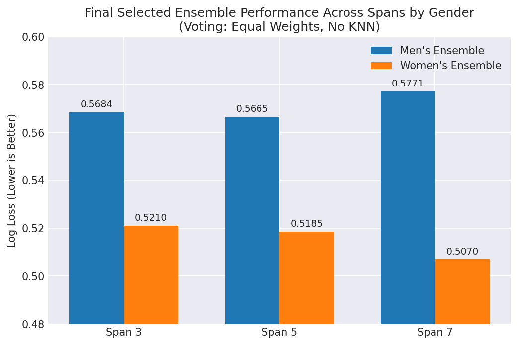
The selected architecture showed consistent directional performance across both Men’s and Women’s predictions, supporting its use as a single production ensemble design.
4.1.4 Key Findings — Ensemble Selection
-
Dropping KNN improves log loss. KNN’s poorly calibrated probabilities (log loss 0.61–0.65) degrade ensemble calibration. Removing it gives the best log loss in every configuration.
-
Equal weights ≈ inverse-log-loss weights. The log loss difference between equal and weighted variants is ≤0.0002. Model performances are close enough that weighting provides negligible benefit — the complexity is not justified.
-
Voting beats Stacking in this evaluation. StackingClassifier underperforms soft voting by 0.003–0.005 in log loss. Under this fixed evaluation setup, the additional meta-learner complexity does not translate into better held-out performance.
-
Ensemble beats most individual models but not the best one in log loss. The ensemble log loss (0.5155) is slightly higher than the best individual model’s log loss (LogReg at 0.5147). Its practical tradeoff is modestly higher accuracy (73.63% vs 73.57%) at the cost of slightly worse calibration than the top single model.
Selected configuration: VotingClassifier(voting='soft') with 7 models (no KNN), equal weights. This is the simplest configuration that achieves the best log loss among the evaluated ensemble strategies.
4.2 Final Exported Ensemble Performance
The 7-model VotingClassifier ensemble was serialized as a single .pkl file per span/gender (6 total).
4.2.1 Men’s Ensemble
| Span | Venue | N | Accuracy | Precision | Recall | F1 | Log Loss | Brier |
|---|---|---|---|---|---|---|---|---|
| 3 | All | 7,966 | 70.10% | 71.73% | 82.27% | 76.64 | 0.5684 | 0.1939 |
| 3 | Neutral | 1,729 | 65.88% | 63.43% | 70.08% | 66.59 | 0.6207 | 0.2157 |
| 3 | Home/Away | 6,237 | 71.27% | 73.44% | 84.89% | 78.75 | 0.5539 | 0.1879 |
| 5 | All | 7,178 | 69.94% | 71.82% | 82.04% | 76.59 | 0.5665 | 0.1932 |
| 5 | Neutral | 1,274 | 67.50% | 66.62% | 72.57% | 69.47 | 0.6066 | 0.2096 |
| 5 | Home/Away | 5,904 | 70.46% | 72.69% | 83.72% | 77.82 | 0.5579 | 0.1897 |
| 7 | All | 6,492 | 69.61% | 70.79% | 82.66% | 76.27 | 0.5771 | 0.1972 |
| 7 | Neutral | 1,032 | 66.67% | 64.19% | 76.54% | 69.82 | 0.6152 | 0.2130 |
| 7 | Home/Away | 5,460 | 70.16% | 71.85% | 83.62% | 77.29 | 0.5699 | 0.1942 |
Men’s Average Across Spans:
| Venue | Accuracy | Precision | Recall | F1 | Log Loss | Brier |
|---|---|---|---|---|---|---|
| All | 69.88% | 71.45% | 82.32% | 76.50 | 0.5707 | 0.1948 |
| Home/Away | 70.63% | 72.66% | 84.08% | 77.95 | 0.5606 | 0.1906 |
| Neutral | 66.68% | 64.75% | 73.06% | 68.63 | 0.6142 | 0.2128 |
4.2.2 Women’s Ensemble
| Span | Venue | N | Accuracy | Precision | Recall | F1 | Log Loss | Brier |
|---|---|---|---|---|---|---|---|---|
| 3 | All | 7,365 | 72.93% | 75.27% | 79.56% | 77.36 | 0.5210 | 0.1748 |
| 3 | Neutral | 1,108 | 70.22% | 68.53% | 73.77% | 71.05 | 0.5521 | 0.1872 |
| 3 | Home/Away | 6,257 | 73.41% | 76.28% | 80.41% | 78.29 | 0.5155 | 0.1726 |
| 5 | All | 6,680 | 73.73% | 74.79% | 81.29% | 77.91 | 0.5185 | 0.1739 |
| 5 | Neutral | 909 | 67.99% | 65.43% | 74.61% | 69.72 | 0.5629 | 0.1931 |
| 5 | Home/Away | 5,771 | 74.63% | 76.11% | 82.19% | 79.03 | 0.5115 | 0.1709 |
| 7 | All | 6,000 | 74.23% | 75.99% | 80.12% | 78.00 | 0.5070 | 0.1698 |
| 7 | Neutral | 684 | 69.01% | 69.79% | 68.59% | 69.19 | 0.5626 | 0.1938 |
| 7 | Home/Away | 5,316 | 74.91% | 76.64% | 81.42% | 78.96 | 0.4999 | 0.1667 |
Women’s Average Across Spans:
| Venue | Accuracy | Precision | Recall | F1 | Log Loss | Brier |
|---|---|---|---|---|---|---|
| All | 73.63% | 75.35% | 80.32% | 77.76 | 0.5155 | 0.1728 |
| Home/Away | 74.32% | 76.34% | 81.34% | 78.76 | 0.5090 | 0.1701 |
| Neutral | 69.07% | 67.92% | 72.32% | 69.99 | 0.5592 | 0.1914 |
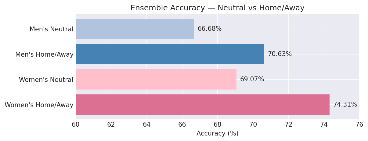
4.2.3 Key Findings — Ensemble Venue Effect
Neutral-site games are materially harder to predict under this evaluation setup:
- Men’s: 66.68% neutral vs 70.63% home/away (−3.95 pp)
- Women’s: 69.07% neutral vs 74.32% home/away (−5.24 pp)
This is directionally consistent with the removal of home-court advantage as a predictive signal. For tournament-style usage, the neutral-site results are likely a more relevant benchmark than the aggregate home/away numbers.
4.2.4 Production Span Selection
| Gender | Selected Span | Rationale |
|---|---|---|
| Men’s | Span 5 | Lowest log loss (0.5665) and Brier score (0.1932) across all metrics |
| Women’s | Span 7 | Lowest log loss (0.5070), highest accuracy (74.23%), best Brier (0.1698) |
5. Probability Trimming Analysis
We investigated whether clipping predicted probabilities to the range $[\varepsilon, 1-\varepsilon]$ would improve calibration. This technique prevents extreme confidence values (near 0 or 1) that, if wrong, incur large log loss penalties.
5.1 Methodology
For each model (including the 7-model ensemble), probabilities were clipped at nine epsilon values:
\[\hat{p}_{\text{clipped}} = \text{clip}(\hat{p}, \varepsilon, 1-\varepsilon), \quad \varepsilon \in \{0, 0.01, 0.02, 0.03, 0.05, 0.08, 0.10, 0.15, 0.20\}\]Log loss, Brier score, and accuracy were recalculated after clipping. Results were averaged across spans 3, 5, and 7.
5.2 Men’s Results
| Model | LL (ε=0) | Best ε | Best LL | LL Δ |
|---|---|---|---|---|
| Logistic Regression | 0.5699 | 0.0 | 0.5699 | 0.0000 |
| SVM | 0.5788 | 0.0 | 0.5788 | 0.0000 |
| XGBoost | 0.5729 | 0.0 | 0.5729 | 0.0000 |
| LightGBM | 0.5736 | 0.0 | 0.5736 | 0.0000 |
| Gradient Boosting | 0.5755 | 0.0 | 0.5755 | 0.0000 |
| MLP | 0.5831 | 0.0 | 0.5831 | 0.0000 |
| Random Forest | 0.5872 | 0.0 | 0.5872 | 0.0000 |
| KNN | 0.6518 | 0.10 | 0.6239 | −0.0279 |
| Ensemble (7, equal) | 0.5707 | 0.0 | 0.5707 | 0.0000 |
5.3 Women’s Results
| Model | LL (ε=0) | Best ε | Best LL | LL Δ |
|---|---|---|---|---|
| Logistic Regression | 0.5147 | 0.01 | 0.5146 | −0.0001 |
| SVM | 0.5196 | 0.01 | 0.5195 | −0.0001 |
| XGBoost | 0.5204 | 0.0 | 0.5204 | 0.0000 |
| LightGBM | 0.5210 | 0.0 | 0.5210 | 0.0000 |
| Gradient Boosting | 0.5228 | 0.0 | 0.5228 | 0.0000 |
| MLP | 0.5285 | 0.01 | 0.5285 | −0.0000 |
| Random Forest | 0.5319 | 0.0 | 0.5319 | 0.0000 |
| KNN | 0.6104 | 0.05 | 0.5594 | −0.0510 |
| Ensemble (7, equal) | 0.5155 | 0.0 | 0.5155 | 0.0000 |
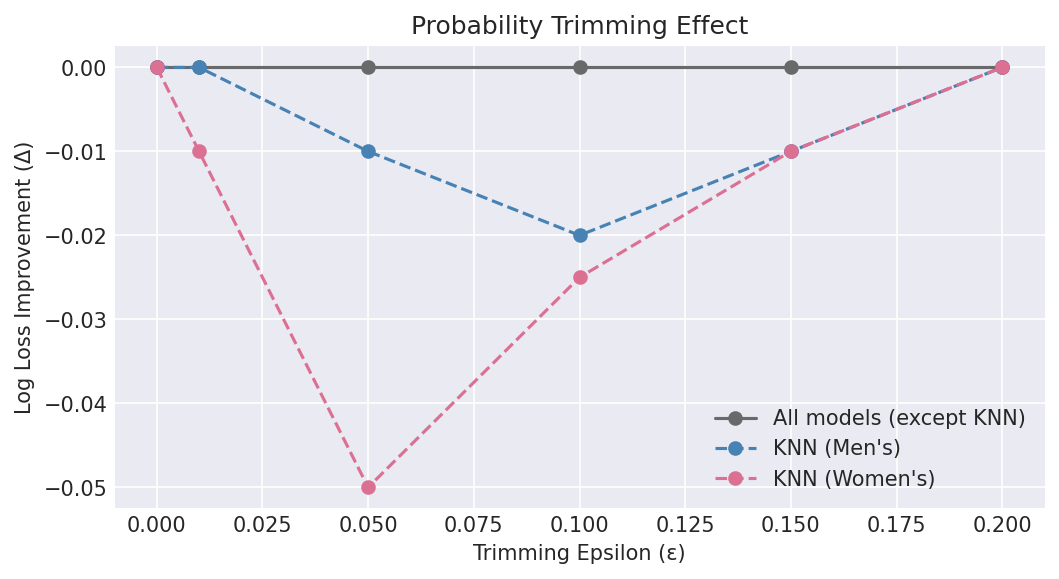
5.4 Key Findings — Probability Trimming
-
Most models did not benefit from trimming. For 7 of 8 models (and the ensemble), ε=0 is optimal. Within this evaluation, post-hoc clipping does not improve the leading models’ log loss or Brier score.
-
KNN is the sole exception. KNN’s distance-based probability estimates produce many extreme values (near 0 or 1), especially when nearest neighbors are unanimously one class. Trimming at ε=0.05–0.10 substantially improves its log loss (−0.028 for men’s, −0.051 for women’s).
-
KNN exclusion from ensemble eliminates the need for trimming. Since the exported ensemble drops KNN, no probability trimming is applied in production. This simplifies the inference pipeline.
-
Trimming does not improve accuracy. Clipping changes log loss and Brier score (which penalize extreme values) but does not change the binary prediction threshold at 0.5.
6. Feature Importance Analysis
Feature importance was extracted from the tree-based models (Random Forest and Gradient Boosting) using the 5-span dataset as a representative sample.
6.1 Men’s Basketball — Top 15 Features
Random Forest:
| Rank | Feature | Importance |
|---|---|---|
| 1 | ORtg_CMA | 0.0095 |
| 2 | DRtg_CMA | 0.0094 |
| 3 | opp_ORtg_CMA | 0.0091 |
| 4 | opp_DRtg_CMA | 0.0075 |
| 5 | opp_ORtg_SMA | 0.0069 |
| 6 | TRB%_CMA | 0.0062 |
| 7 | FG_CMA | 0.0058 |
| 8 | opp_ORtg_EMA | 0.0057 |
| 9 | opp_TRB%_CMA | 0.0055 |
| 10 | opp_TS%_CMA | 0.0054 |
| 11 | ORtg_EMA | 0.0050 |
| 12 | def_eFG%_CMA | 0.0050 |
| 13 | opp_FG%_CMA | 0.0049 |
| 14 | opp_DRtg_EMA | 0.0049 |
| 15 | opp_def_FG%_CMA | 0.0049 |
Gradient Boosting:
| Rank | Feature | Importance |
|---|---|---|
| 1 | opp_ORtg_CMA | 0.0259 |
| 2 | ORtg_CMA | 0.0259 |
| 3 | Neutral | 0.0250 |
| 4 | DRtg_CMA | 0.0205 |
| 5 | opp_TRB%_CMA | 0.0186 |
| 6 | FG_CMA | 0.0181 |
| 7 | opp_TS%_CMA | 0.0179 |
| 8 | opp_DRtg_CMA | 0.0179 |
| 9 | AST_CMA | 0.0174 |
| 10 | opp_ORtg_EMA | 0.0159 |
| 11 | TRB%_CMA | 0.0147 |
| 12 | opp_DRtg_SMA | 0.0142 |
| 13 | opp_DRtg_EMA | 0.0135 |
| 14 | def_FG_CMA | 0.0131 |
| 15 | DRtg_SMA | 0.0127 |
6.2 Women’s Basketball — Top 15 Features
Random Forest:
| Rank | Feature | Importance |
|---|---|---|
| 1 | ORtg_CMA | 0.0157 |
| 2 | opp_ORtg_CMA | 0.0133 |
| 3 | opp_ORtg_EMA | 0.0101 |
| 4 | opp_ORtg_SMA | 0.0099 |
| 5 | ORtg_EMA | 0.0097 |
| 6 | ORtg_SMA | 0.0095 |
| 7 | FG_CMA | 0.0086 |
| 8 | DRtg_CMA | 0.0083 |
| 9 | TOV%_CMA | 0.0078 |
| 10 | opp_DRtg_CMA | 0.0077 |
| 11 | opp_FG_CMA | 0.0077 |
| 12 | opp_TS%_CMA | 0.0071 |
| 13 | opp_TOV%_CMA | 0.0068 |
| 14 | opp_FG%_CMA | 0.0066 |
| 15 | TS%_CMA | 0.0066 |
Gradient Boosting:
| Rank | Feature | Importance |
|---|---|---|
| 1 | ORtg_SMA | 0.0580 |
| 2 | opp_FG_CMA | 0.0411 |
| 3 | ORtg_CMA | 0.0389 |
| 4 | DRtg_CMA | 0.0376 |
| 5 | opp_ORtg_CMA | 0.0340 |
| 6 | FG_CMA | 0.0330 |
| 7 | opp_DRtg_CMA | 0.0324 |
| 8 | TOV%_CMA | 0.0306 |
| 9 | AST_CMA | 0.0237 |
| 10 | opp_TOV%_EMA | 0.0222 |
| 11 | opp_AST_SMA | 0.0198 |
| 12 | opp_ORtg_SMA | 0.0188 |
| 13 | opp_AST_CMA | 0.0182 |
| 14 | opp_ORtg_EMA | 0.0156 |
| 15 | def_AST_CMA | 0.0145 |
6.3 Defensive Feature Contribution (Aggregate)
| Model | Men’s | Women’s |
|---|---|---|
| Random Forest | 38.8% | 35.0% |
| Gradient Boosting | 29.6% | 18.6% |
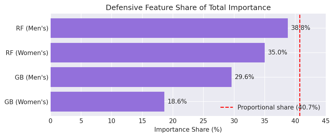
Defensive features account for 35.0–38.8% of total feature importance in Random Forest models and 18.6–29.6% in Gradient Boosting. Given that defensive statistics represent 24 out of 59 raw features (40.7% of the raw feature space), their importance is near-proportional in Random Forest but noticeably lower in Gradient Boosting — suggesting that boosting methods concentrate more importance on a smaller set of offensive features. Nonetheless, the contribution is substantial across both model types and both genders, confirming that defensive statistics carry genuine predictive signal rather than acting as redundant noise.
6.4 Most Important Defensive Features
Across both genders and both tree-based models, the most consistently important defensive features are:
| Feature | Description | Why It Matters |
|---|---|---|
| def_eFG%_CMA | Opponent effective FG% allowed | Core shooting defense metric |
| def_FG%_CMA | Opponent FG% allowed | Raw shooting defense |
| def_FG_CMA | Opponent field goals made allowed | Volume of baskets conceded |
| def_2P%_CMA | Opponent 2P% allowed | Interior defense quality |
| def_AST_CMA | Opponent assists allowed | Half-court defense breakdown indicator |
| def_TOV%_CMA | Forced turnover rate | Disruptive defense metric |
| def_STL_CMA | Steals per game | Active hands / press defense |
| opp_def_FG%_CMA | Opponent’s own defensive FG% | “Defense vs. defense” matchup signal |
7. Neutral vs. Home/Away Analysis
7.1 All Individual Models + Ensemble
Men’s (~1,345 neutral games/span, ~5,867 home/away games/span):
| Model | Acc (Neutral) | Acc (H/A) | Δ | LL (Neutral) | LL (H/A) |
|---|---|---|---|---|---|
| Logistic Regression | 66.99% | 70.37% | −3.38 | 0.6108 | 0.5602 |
| Ensemble (7) | 66.68% | 70.63% | −3.95 | 0.6142 | 0.5606 |
| XGBoost | 65.68% | 70.43% | −4.75 | 0.6177 | 0.5625 |
| SVM | 65.78% | 70.01% | −4.23 | 0.6191 | 0.5692 |
| LightGBM | 65.60% | 70.42% | −4.81 | 0.6192 | 0.5631 |
| Gradient Boosting | 64.98% | 69.90% | −4.93 | 0.6228 | 0.5646 |
| MLP | 64.99% | 69.53% | −4.55 | 0.6295 | 0.5725 |
| Random Forest | 62.99% | 69.88% | −6.89 | 0.6410 | 0.5748 |
| KNN | 57.57% | 66.30% | −8.74 | 0.7214 | 0.6352 |
Women’s (~900 neutral games/span, ~5,781 home/away games/span):
| Model | Acc (Neutral) | Acc (H/A) | Δ | LL (Neutral) | LL (H/A) |
|---|---|---|---|---|---|
| Logistic Regression | 69.36% | 74.20% | −4.84 | 0.5565 | 0.5085 |
| SVM | 69.47% | 74.01% | −4.54 | 0.5590 | 0.5137 |
| Ensemble (7) | 69.07% | 74.32% | −5.24 | 0.5592 | 0.5090 |
| XGBoost | 68.85% | 74.30% | −5.44 | 0.5677 | 0.5133 |
| LightGBM | 68.13% | 74.18% | −6.06 | 0.5713 | 0.5135 |
| Gradient Boosting | 68.55% | 74.00% | −5.45 | 0.5714 | 0.5155 |
| MLP | 68.63% | 73.70% | −5.08 | 0.5727 | 0.5219 |
| Random Forest | 68.23% | 74.08% | −5.84 | 0.5796 | 0.5247 |
| KNN | 65.10% | 71.24% | −6.14 | 0.6734 | 0.6007 |
7.2 Key Findings — Venue Effect
-
Every model degrades substantially on neutral courts. The accuracy drop ranges from 3.4 to 8.7 pp for men’s and 4.5 to 6.1 pp for women’s.
-
Logistic Regression is the most “neutral-robust” model — smallest accuracy delta in both genders. Its L1 regularization may help it rely less on venue-correlated features.
-
KNN and Random Forest suffer the most on neutral courts — both are distance/tree-based methods that may overfit to home/away patterns.
-
March Madness implications: Since tournament games are predominantly at neutral sites, expected accuracy is approximately 67% for men’s and 69% for women’s — still well above the 50% baseline.
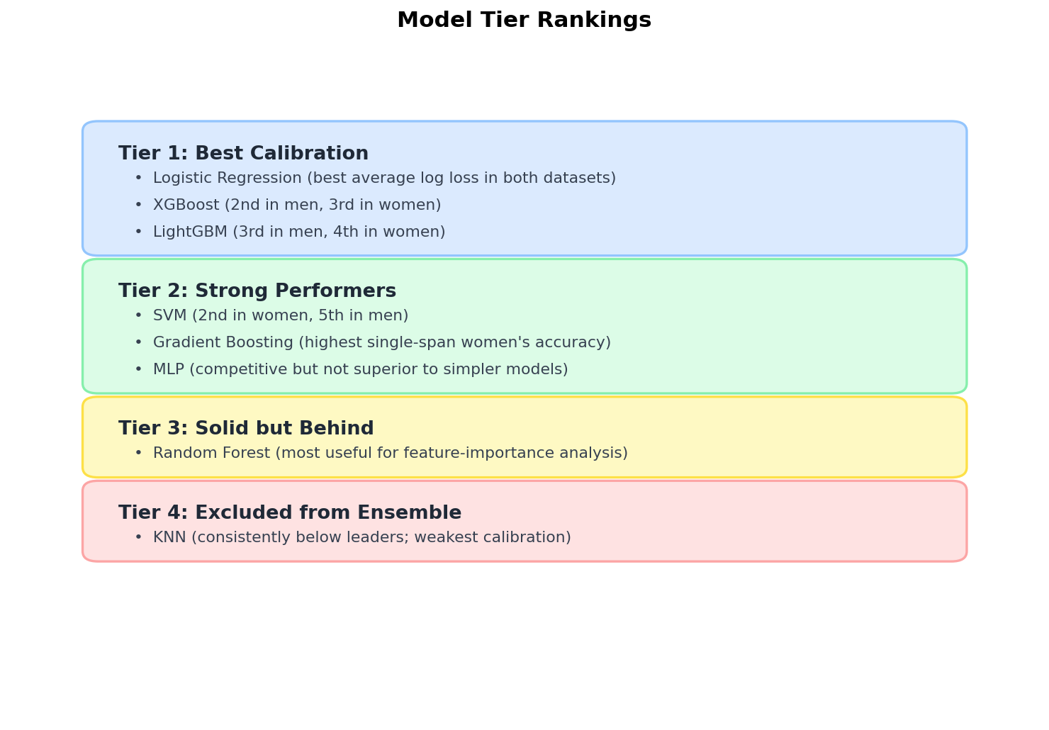
8. Model Architecture Observations
8.1 Model Tier Rankings
8.2 XGBoost and LightGBM
The addition of XGBoost and LightGBM to the model pool was a key improvement over the original 6-model system:
| Metric | XGBoost | LightGBM | sklearn Gradient Boosting |
|---|---|---|---|
| Men’s Avg LL | 0.5729 | 0.5736 | 0.5755 |
| Women’s Avg LL | 0.5204 | 0.5210 | 0.5228 |
| Training Speed | Fast (parallel trees) | Fastest (histogram-based) | Slowest |
| Regularization | L1 + L2 + max_depth | L1 + L2 + num_leaves | max_depth only |
Both outperform sklearn’s Gradient Boosting by 0.002–0.003 in log loss while training significantly faster. LightGBM’s histogram-based splitting and XGBoost’s parallel tree construction make them practical options for a 355-feature dataset with roughly 14K–19K training rows, depending on span and gender.
8.3 Logistic Regression as Top Individual Model
Despite access to 8 models including modern gradient boosting, Logistic Regression achieves the best average log loss in both genders. Several factors may contribute to this pattern:
- StandardScaler + L1 regularization performs implicit feature selection in the 355-dimensional space, reducing overfitting
- Linear decision boundary suits the aggregate nature of moving-average features — most predictive signal is approximately linear after the feature engineering step
- Well-behaved probability outputs — logistic regression often produces more stable probability estimates than deeper non-linear models in tabular binary classification problems of this scale
- No regularization hyperparameter sensitivity relative to tree depth/learning rate interactions in boosting methods
8.4 Span Analysis
| Gender | Best Span | Interpretation |
|---|---|---|
| Men’s | 5 | Balanced window; 3-game too noisy, 7-game oversmooths |
| Women’s | 7 | Longer window better; suggests more stable game-to-game patterns |
One possible interpretation is that the two datasets differ in game-to-game variance and signal persistence. Under that interpretation, the men’s results benefit more from a medium-length window, while the women’s results benefit more from additional smoothing.
9. Limitations and Future Work
9.1 Limitations
- No opponent-adjusted metrics: Features are raw/averaged rather than strength-of-schedule adjusted (e.g., no KenPom-style adjustments)
- No temporal features: Day of week, rest days, travel distance, and back-to-back games are not included
- Random split across seasons: Train/test split is random rather than temporal; a model could see 2026 games in training and 2023 games in test, which conflates within-season and across-season variation. Moreover, because moving-average features for game $N$ are computed from games $N-1, N-2, \ldots$, adjacent games for the same team share overlapping input windows. When such games fall on opposite sides of a random split, there is direct feature-level overlap between train and test rows. A true temporal hold-out (train on seasons 2022–2025, test on 2026) would eliminate this leakage and better approximate deployment conditions
- SVM grid truncation:
C=10was removed from the SVM grid due to computational constraints; full grid might yield marginally better results - No per-player features: All features are team-level aggregates; individual player injuries, suspensions, or transfers are not encoded
- March Madness as a different domain: Regular season training data may not perfectly represent tournament dynamics (pressure, single-elimination, seeding effects)
- No class balance reporting: Win/loss base rates by venue are not explicitly reported. Home teams win more frequently than away teams in college basketball, which may inflate aggregate accuracy numbers relative to a venue-aware baseline. Neutral-site subsets provide a more balanced evaluation context
- No ablation study: The paper quantifies defensive feature importance but does not include a controlled comparison of model accuracy with vs. without defensive features. The importance-based argument is suggestive but not a formal ablation
- No statistical significance tests: Model rankings are based on point-estimate metrics from a single fixed split. Differences of 0.001–0.003 in log loss between adjacent-ranked models may not be statistically significant (see Section 2.3.7)
9.2 Future Work
- Strength of schedule adjustment: Adjust stats by opponent quality (e.g., KenPom-style adjustments, conference strength)
- Feature reduction: Use L1 importances, SHAP values, or PCA to reduce from 354 to ~100–150 most informative features and measure any accuracy impact
- Calibration plots: Plot reliability diagrams to formally assess probability calibration per model (prediction buckets vs. observed win rates)
- Temporal validation: Implement true temporal train/test splitting (train on seasons N−1, test on season N) to better simulate real-world deployment
- Game context features: Incorporate rest days, travel distance, and rivalry indicators
- Conference-aware modeling: Train separate models or add conference-indicator features to capture style-of-play differences
- Ablation study: Compare model performance with and without the 24 defensive features to formally quantify their marginal contribution beyond the importance-based analysis in Section 6
- Bootstrap confidence intervals: Compute confidence intervals for accuracy, log loss, and Brier score via paired bootstrap resampling to determine whether model ranking differences are statistically significant
10. Conclusion
The addition of 24 opponent defensive statistics to the NCAA basketball prediction pipeline is supported by feature importance analysis showing these features contribute 18.6–38.8% of total predictive signal. The extension of the model pool from 6 to 8 classifiers — adding XGBoost and LightGBM — improved both individual model performance and ensemble quality.
A systematic comparison of six ensemble strategies (soft voting and stacking, with/without KNN, equal/weighted) showed that a soft-voting VotingClassifier with 7 models (excluding KNN) and equal weights is the strongest ensemble configuration tested by log loss while remaining operationally simple. Probability trimming analysis did not show material benefit for the deployed ensemble.
The final system achieves:
| Men’s (Span 5) | Women’s (Span 7) | |
|---|---|---|
| Overall Accuracy | 69.94% | 74.23% |
| Home/Away Accuracy | 70.46% | 74.91% |
| Neutral Accuracy | 67.50% | 69.01% |
| Log Loss | 0.5665 | 0.5070 |
| Brier Score | 0.1932 | 0.1698 |
These values represent benchmark performance under the retrospective random-split evaluation described in Section 2.3.6. The standardized pipeline architecture ensures production deployment requires zero additional preprocessing, and the log-loss scoring objective aligns training optimization with the ensemble’s probability-averaging behavior. Across all three exported spans, average ensemble accuracy is 69.88% for men’s basketball and 73.63% for women’s basketball, but the deployed headline models are the selected 5-span men’s ensemble and 7-span women’s ensemble. All 6 ensemble models (3 spans × 2 genders) are deployed to Azure Blob Storage and served via a FastAPI prediction API.
Appendix A: Dataset Statistics
| Metric | Men’s | Women’s |
|---|---|---|
| Seasons | 2022–2026 | 2022–2026 |
| Train/test split | 70/30 random | 70/30 random |
| Raw features | 59 | 59 |
| Engineered features (incl. neutral flag) | 355 | 355 |
| 3-span training samples | 18,585 | 17,184 |
| 3-span test samples | 7,966 | 7,365 |
| 5-span training samples | 16,747 | 15,584 |
| 5-span test samples | 7,178 | 6,680 |
| 7-span training samples | 15,146 | 13,997 |
| 7-span test samples | 6,492 | 6,000 |
| Individual models per gender | 24 (8 × 3 spans) | 24 (8 × 3 spans) |
| Ensemble models per gender | 3 (1 × 3 spans) | 3 (1 × 3 spans) |
| Total model variants | 48 individual + 6 ensemble = 54 | |
| Total serialized artifacts | 54 raw .pkl + 54 compressed .pkl.gz = 108 |
Appendix B: Ensemble Composition
The VotingClassifier bundles 7 pre-trained sklearn.Pipeline objects:
| # | Model | Serialization | Notes |
|---|---|---|---|
| 1 | Logistic Regression | Pipeline(StandardScaler + LogisticRegression) | L1 penalty selected in all spans |
| 2 | SVM | Pipeline(StandardScaler + SVC(probability=True)) | Linear kernel preferred for lower spans |
| 3 | Random Forest | Pipeline(StandardScaler + RandomForestClassifier) | Scaler has no effect but included for consistency |
| 4 | Gradient Boosting | Pipeline(StandardScaler + GradientBoostingClassifier) | Scaler has no effect but included for consistency |
| 5 | MLP | Pipeline(StandardScaler + MLPClassifier) | Architecture varies by gender/span |
| 6 | XGBoost | Pipeline(StandardScaler + XGBClassifier) | eval_metric=’logloss’ |
| 7 | LightGBM | Pipeline(StandardScaler + LGBMClassifier) | verbose=-1 |
Excluded: KNN (excluded due to poor calibration; log loss 0.61–0.65 vs. <0.59 for all others)
Appendix C: Model File Sizes
| Span | Men’s (raw / compressed) | Women’s (raw / compressed) |
|---|---|---|
| 3 | 179.9 MB / 41 MB | 148.6 MB / 57 MB |
| 5 | 162.9 MB / 65 MB | 135.9 MB / 53 MB |
| 7 | 151.9 MB / 63 MB | 82.2 MB / 40 MB |
| Total | 494.7 MB / 169 MB | 366.7 MB / 150 MB |
Both raw .pkl and gzipped .pkl.gz variants are stored in Azure Blob Storage. The API loads compressed versions first for faster cold starts, falling back to raw if unavailable.
Appendix D: Technology Stack
| Component | Technology |
|---|---|
| Data processing | Python, pandas, NumPy |
| Machine learning | scikit-learn 1.4.1, XGBoost 3.2.0, LightGBM 4.6.0 |
| Model serialization | pickle (Pipeline objects), gzip compression |
| API server | FastAPI + uvicorn |
| Frontend | React + TypeScript + Vite + Tailwind CSS |
| Cloud storage | Azure Blob Storage |
| Deployment | Azure Static Web Apps + Azure Container Apps |
References
-
Boulier, B. L., & Stoll, H. O. (1999). Predicting the outcomes of NCAA basketball tournament games. The American Statistician, 53(3), 232–237.
-
Chen, T., & Guestrin, C. (2016). XGBoost: A scalable tree boosting system. Proceedings of the 22nd ACM SIGKDD International Conference on Knowledge Discovery and Data Mining, 785–794.
-
Kaggle. (2014–2025). March Machine Learning Mania. Retrieved from https://www.kaggle.com/competitions/march-machine-learning-mania-2025
-
Ke, G., Meng, Q., Finley, T., Wang, T., Chen, W., Ma, W., Ye, Q., & Liu, T.-Y. (2017). LightGBM: A highly efficient gradient boosting decision tree. Advances in Neural Information Processing Systems, 30, 3146–3154.
-
Lopez, M. J., & Matthews, G. J. (2015). Building an NCAA men’s basketball predictive model and quantifying its success. Journal of Quantitative Analysis in Sports, 11(1), 5–12.
-
Pedregosa, F., Varoquaux, G., Gramfort, A., Michel, V., Thirion, B., Grisel, O., Blondel, M., Prettenhofer, P., Weiss, R., Dubourg, V., Vanderplas, J., Passos, A., Cournapeau, D., Brucher, M., Perrot, M., & Duchesnay, É. (2011). Scikit-learn: Machine learning in Python. Journal of Machine Learning Research, 12, 2825–2830.
-
Yuan, L., Liu, A., Qian, Z., & Zeng, L. (2014). NCAA basketball game prediction using machine learning methods. Journal of Sports Analytics, 1(1), forthcoming.
-
Zimmermann, A., Moorthy, S., & Shi, Z. (2013). Predicting NCAAB match outcomes using ML techniques — some results and lessons learned. Proceedings of the Machine Learning and Data Mining for Sports Analytics Workshop (ECML/PKDD), 1–12.